Case Study: Mapping German ZIP Codes in R

Shortly after running a webinar last week I received an email from Achim Rumberger, who attended the webinar live. Achim immediately put the webinar material into use for his own project, which involves mapping ZIP Codes in Germany. This was the first case study I received related to my new course, Shapefiles for R Programmersand I wanted to share it with my readers.

I’m neuro-biologist by training, but for the past decade I make my living as a JAVA enterprise developer. I’m living and working in Germany, near Stuttgart, where Mercedes Benz cars and Porsches are manufactured.

Recently my daughter came to me with a problem – for her bachelor thesis she wants to see if certain kind of schools will benefit from the help of social services. So I suggested to her, to look for public available data, describing the social structure of the environment of these schools in question.

And all of a sudden, there was the problem to show some data in a geographical context.

Just at this time Ari published his webinar about getting shape files into R. Which also includes a introduction to shape files to get you going, if you are new to it, as I am. I remembered Ari from his mail course introducing his great R-package (choroplethr). By the way this is a terrible name, being a biologist by heart, I always type “chloroplethr”, as in “chlorophyll”, and this is not found by the R package manager. [Editor’s note: I agree!]

Next question, where do I get the shapefiles, describing Germany? A major search engine was of great help here. http://www.suche-postleitzahl.org/downloads?download=zuordnung_plz_ort.csv . Germany has some 8700 zip code areas, so expect some time for rendering the file, if you do on your computer. Right on this side one can also find a dataset which might act as a useful warm up practice to display statistical data in a geographical context. Other sources are https://datahub.io/de/dataset/postal-codes-de

And so I got started…

For development in R, I’m using RStudio, as its free, and most closely resembles the IDEs I know from JAVA development, though its functionality is a throwback to the 90s, compared to modern IDEs like Netbeans or IntelliJ. Especially in respect to refactoring and debugging.

To complete this task, there are whole lot of packages needed. But these will make life a whole lot easier. Look for the most recent packages, especially “readr”, which helps with loading the csv files into R. With “readr” you do not have to convert factors in strings again, as it is the case with the readcsv function from R.

The code itself is mostly copied and pasted from Ari’s webinar. It basically loads the shapefile into R, converts it into a data.frame and provides this data.frame with a variable called “region”. Then the stat data is loaded into R, again, the columns are renamed to something “choroplethr” recognizes (“region” and “values”), and finally “choroplethr” its doing it magic.

[content_upgrade cu_id=”2693″]Bonus: Download the code from this post![content_upgrade_button]Download[/content_upgrade_button][/content_upgrade]

My hardware used is a MacBook from 2011 with 16GB RAM and an i7 Processor. The execution time for each of the plots is around 5 mins. R is using only a single core of the 4 available, but big memory helps.

And here is the code:

#make sure the workspace is in pristine condition
rm(list=ls(all=TRUE))
#shapefile from https://datahub.io/de/dataset/postal-codes-de
#http://www.suche-postleitzahl.org/downloads?download=zuordnung_plz_ort.csv
#post questions here: http://gis.stackexchange.com/
library(choroplethr)
library(dplyr)
library(ggplot2)
library(rgdal)
library(maptools)
library(gpclib)
library(readr)
library(R6)
setwd("<path to your shape file>/plz-gebiete.shp/")
ger_plz <- readOGR(dsn = ".", layer = "plz-gebiete")
gpclibPermit()
#convert the raw data to a data.frame as ggplot works on data.frames
ger_plz@data$id <- rownames(ger_plz@data)
ger_plz.point <- fortify(ger_plz, region="id")
ger_plz.df <- inner_join(ger_plz.point,ger_plz@data, by="id")
head(ger_plz.df)
ggplot(ger_plz.df, aes(long, lat, group=group )) + geom_polygon()
#data file
df <- read_csv("<path to your stat data>/de_plz_einwohner.csv")
# variable name 'region' is needed for choroplethr
ger_plz.df$region <- ger_plz.df$plz
head(ger_plz.df)
#subclass choroplethr to make a class for your my need
GERPLZChoropleth <- R6Class("GERPLZChoropleth",
    inherit = choroplethr:::Choropleth,
    public = list(
        initialize = function(user.df) {
            super$initialize(ger_plz.df, user.df)
        }
    )
)
#choropleth needs these two columnames - 'region' and 'value'
colnames(df) = c("region", "value")
#instantiate new class with data
c <- GERPLZChoropleth$new(df)
#plot the data
c$ggplot_polygon = geom_polygon(aes(fill = value), color = NA)
c$title = "Comparison of number of Inhabitants per Zipcode in Germany"
c$legend= "Number of Inhabitants per Zipcode"
c$set_num_colors(9)
c$render()

And here is the result:

What you can see from the map, is that zip codes in the north and east of Germany tend to be larger. Small size zip codes coincide with metropolitan areas in Germany.

ger_zip_codes

Note that with choroplethr, it is easy to combine this choropleth map with a google map. This is useful for people who aren’t already familiar with German geography:

c$render_with_reference_map()

unnamed-1

Update

Due to popular demand of a selected view, here is the result for population density per square kilometer. To do this I had to figure out the area in square km of a zip code. This information is buried deeply in the shapefile structure. But there is an easier way. In QGIS load the shapefile, go to menu “Vector” –> “Geometry-Tools” –> ” Export/Add geometry columns” . Save the output file, and there are the additional columns in the “data” part of the shapefile. There is one thing, the area value of the shapefile has to be multiplied by some factor(12392) to give the value in square km. And here is the code. Have fun.

#copy the original shapefile data.frame
ger_plz4merge <-ger_plz.df
# get rid of columns we don't need
drops <- c("long", "lat", "order", "hole", "piece", "id", "note", "PERIMETER", "group")
ger_plz4merge <- ger_plz4merge[ , !(names(ger_plz4merge) %in% drops)]
#remove duplicates
ger_plz4merge <- unique(ger_plz4merge)
#merge with the population data
df.merge <- join(ger_plz4merge, df, by="plz", type="right", match = "first")
df.merge <- transform(df.merge, AREA2 = AREA*12392)
df.merge <- transform(df.merge, OCC_DENS = einwohner/AREA2)
colnames(df.merge) = c("region", "einwohner","AREA","AREA2", "value")
#now you can use the data as before
c <- GERPLZChoropleth$new(df.merge)

pop_dens_zip_with_ref

[content_upgrade cu_id=”2693″]Bonus: Download the code from this post![content_upgrade_button]Download[/content_upgrade_button][/content_upgrade]

Want to learn how to do projects like this? Take my course Shapefiles for R Programmers.

16 comments
gspiride says May 16, 2016

Awesome summary, thank you Achim.

It would be nice to tie off the story and find out what was the outcome for the question stated in the beginning “look for public available data, describing the social structure of the environment of these schools in question”

    Ari Lamstein says May 16, 2016

    Perhaps Achim (or his daughter 🙂 will be willing to share that analysis when they complete it!

    Achim Rumberger says May 16, 2016

    Happy you liked it, to compile, analyze and publish the data will be the task of my daughter ;^)
    have fun, Achim

Ben says May 17, 2016

Thanks a lot for sharing!!
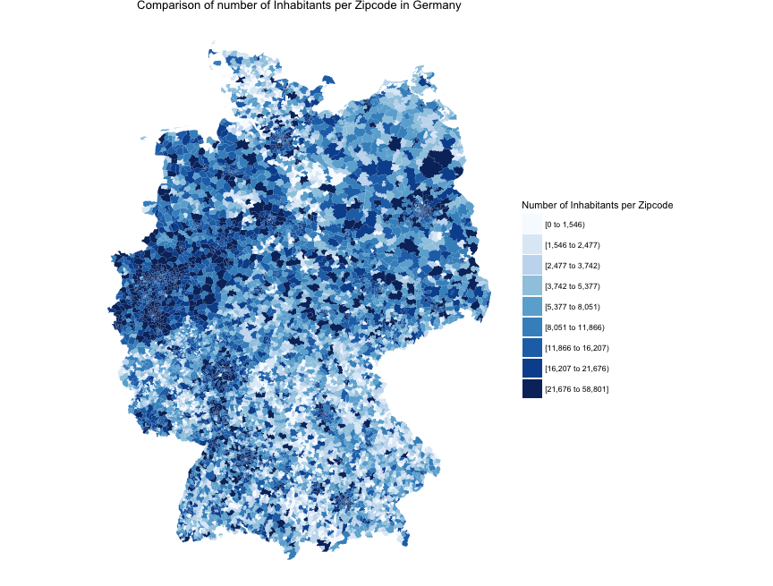
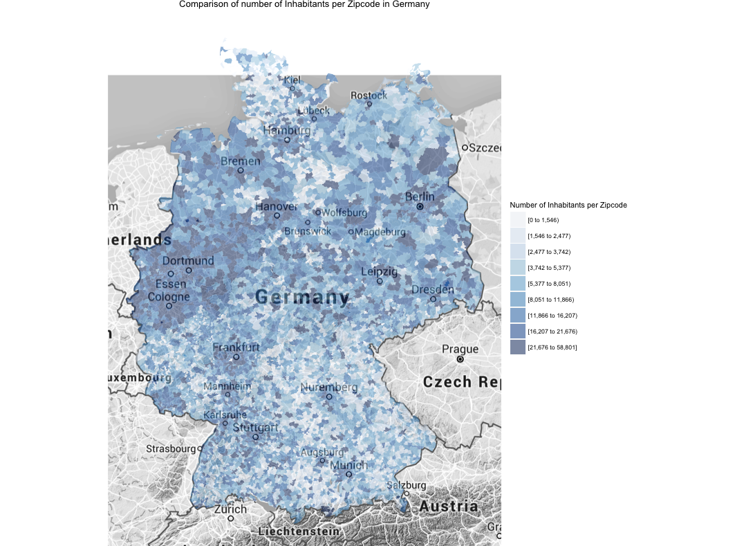
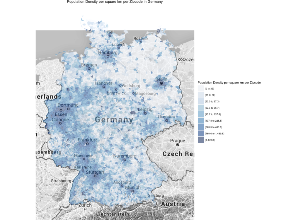
If I understand correctly one can see the number of inhabitants per zip code. Is there a way to also display the density of people per zip code? So the number of inhabitants per m2 of zip code. This would look different since the zip code area size seems to vary a lot wouldn’t it?
I’m also excited about your daughters analysis!
Cheers, Ben

    Ari Lamstein says May 17, 2016

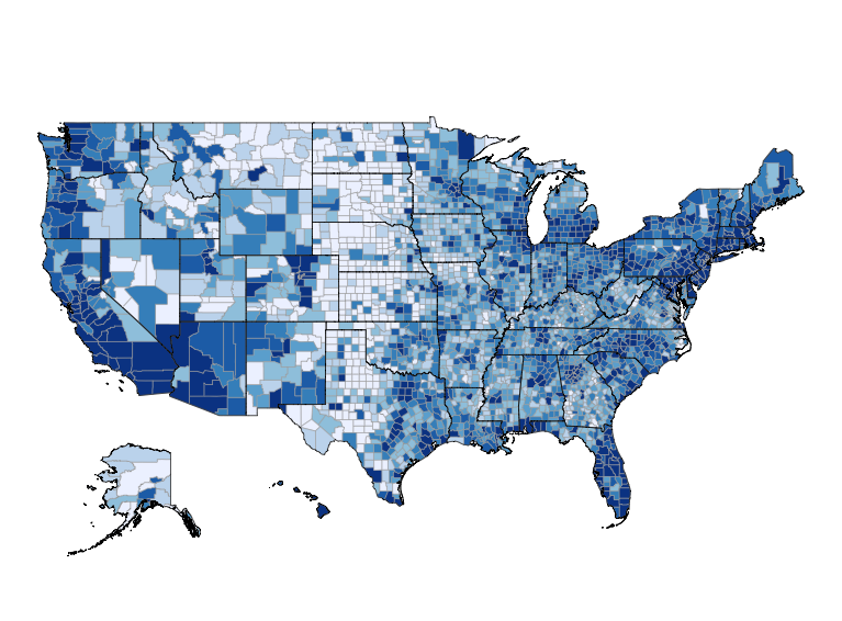
    I don’t know about that shapefile, but the ones from the US Census Bureau also have an “area” column, so it is possible there. See this discussion in the choroplethr google group: https://groups.google.com/forum/#!searchin/choroplethr/density/choroplethr/Z6PmsN7xBiM/6Le7nWXiAwAJ

    Achim Rumberger says May 17, 2016

    Hi Ben.
    Glad you liked my post. You are correct, normalizing the data to inhabitants per m^2 would change the appearance of the map. There is an “area” column buried inside the shapefile structure, I would have to coerce this to change the plot according to your suggestion.
    I also looking forward to my daughter analyses, which may take a while, especially acquiring the data.
    Have fun,
    Achim

gspiride says May 19, 2016

Achim – I’ve just come across NUTS 2 and 3 level charts available from Eurostat in another blog post

Here it is – take a look at the charts, very interesting picture emerging about what sounds like may be tangentially related to your daughter’s original line of inquiry. Might be useful to learn about all the data available to capture various dimensions of the impact of the social structure of the environment that you referred to.

http://www.unz.com/gnxp/europe-on-a-finer-cartographic-scale/?utm_source=rss&utm_medium=rss&utm_campaign=europe-on-a-finer-cartographic-scale

    Achim Rumberger says May 19, 2016

    Thank you GMS – this looks awesome. Generally it seems easier to get this kind of data from EU sources, than from the German “Statische Landesämter”.
    Thanks again, Achim

John says May 24, 2016

Awesome tutorial, thanks a lot. When trying to run your code, I receive an error when instantiating the new class saying that “region” is not a map.df colname. I’m a relative beginner and am not sure where exactly the breaking point is. Has anyone else received this error or knows how to solve it?

    Achim Rumberger says May 24, 2016

    Hi John.
    Glad you liked the post. Sorry you have problems with the example. Do you see this error with the first part of the example, or in the update?
    Have fun, Achim

      John says May 24, 2016

      Hi Achim,

      thanks a lot for getting back on this. I see this error when trying to execute the very first part of the example when line 47 “c <- GERPLZChoropleth$new(df)" should be executed.

      Thanks and best, John

        Achim Rumberger says May 25, 2016

        Hi John,
        perhaps something went wrong here:
        ger_plz.df$region <- ger_plz.df$plz
        this command:
        head(ger_plz.df)
        should give you something like this:
        [code lang="r"]
        long lat order hole piece id group plz note region
        1 5.866315 51.05110 1 FALSE 1 0 0.1 52538 52538 Gangelt, Selfkant 52538
        2 5.866917 51.05124 2 FALSE 1 0 0.1 52538 52538 Gangelt, Selfkant 52538
        [/code]

        have fun
        Achim

Matthias Raess says July 24, 2016

Thanks, Achim (and Ari by extension) for the great tutorial! One more point to note, R likes to throw the following error when trying to join ‘region x region’: Error: Can’t join on ‘region’ x ‘region’ because of incompatible types (integer / factor). This can easily be solved by making sure both region columns in df and ger_plz.df are either integer/factor (as long as they are the same) I solved it with the as.factor() function.

All best,

Matthias

Scott says August 10, 2016

late to the party, but just wanted to say, these are great. thanks

Luis says September 23, 2016

Hi i am a geographer and R spatial coder from Rio de Janeiro..great post very useful code thks!

Tots says November 10, 2016

Hi, i am very new to this so apologies in advance if the question sounds naive. I copied the script in an editor and ran it using the source command in the R console. Everything seems to work fine except i cannot see the map in quartz, the message i am getting after running it is:

OGR data source with driver: ESRI Shapefile
Source: “.”, layer: “plz-gebiete”
with 8712 features
It has 2 fields
Parsed with column specification:
cols(
plz = col_character(),
einwohner = col_integer()
)
Map from URL : http://maps.googleapis.com/maps/api/staticmap?center=50.233703,10.362028&zoom=6&size=640×640&scale=2&maptype=terrain&language=en-EN&sensor=false
Scale for ‘x’ is already present. Adding another scale for ‘x’, which will replace the existing
scale.
Scale for ‘y’ is already present. Adding another scale for ‘y’, which will replace the existing
scale.
Warning messages:
1: In gpclibPermit() :
support for gpclib will be withdrawn from maptools at the next major release
2: In left_join_impl(x, y, by$x, by$y, suffix$x, suffix$y) :
joining character vector and factor, coercing into character vector
3: In left_join_impl(x, y, by$x, by$y, suffix$x, suffix$y) :
joining character vector and factor, coercing into character vector

Any idea why?

Thanks for taking the time to post this code and detail all the steps.

Comments are closed