New R Package for Visualizing California Census Tracts

Today I am happy to announce that my newest R package, choroplethrCaCensusTract, is now available on github. The package’s title is a combination of three words:

  1. choroplethr: the package has similar functions and data objects as my package choroplethr. The name choroplethr itself is a combination of the words choropleth map and R programming language.
  2. Ca: an abbreviation of the US State of California.
  3. census Tracts are geographic units used by the US Census Bureau. Tract boundaries do not change very often and normally contain between 1,200 and 8,000 people.

The package helps you visualize data that is aggregated at the level of census tracts in California. It also helps you to work with demographic data from the US Census Bureau that is aggregated at this level.

Example: Population

# install.packages("devtools")
library(devtools)
install_github("[email protected]", "arilamstein")
library(choroplethrCaCensusTract)
data(df_pop_ca_tract)
?df_pop_ca_tract
?ca_tract_choropleth
ca_tract_choropleth(df_pop_ca_tract, title = "2012 Population Estimates\n California Census Tracts", legend = "Population") + coord_map()


ca-tract-mercator

Note that you can add any projection to this map by using ggplot2’s coord_map() function. Simply add “+ coord_map()” to the above function call.

Because census tracts normally have less than 8,000 people, it is hard to see the tracts in urban areas on a state-wide map.  We can zoom in on individual counties by using the county_zoom parameter. county_zoom takes a vector of County FIPS Codes.

# 6075 is the FIPS code for San Francisco County
ca_tract_choropleth(df_pop_ca_tract,
                    title       = "2012 Population Estimates\n San Francisco Census Tracts",
                    legend      = "Population",
                    county_zoom = 6075) + coord_map()

sf-tract-mercator


I suspect that most people will wonder what the island off the west coast is. It is the Farallon Islands.

Example: Per Capita Income

choroplethrCaCensusTract ships with a data.frame, df_ca_tract_demographics, that has eight demographic variables from the 2013 5-year American Community Survey (ACS).

data(df_ca_tract_demographics)
?df_ca_tract_demographics
colnames(df_ca_tract_demographics)
## [1] "region"            "total_population"  "percent_white"    
## [4] "percent_black"     "percent_asian"     "percent_hispanic" 
## [7] "per_capita_income" "median_rent"       "median_age"
df_ca_tract_demographics$value = df_ca_tract_demographics$per_capita_income
ca_tract_choropleth(df_ca_tract_demographics,
                    title = "2013 San Francisco Census Tracts\n Per Capita Income",
                    legend = "Dollars",
                    num_colors = 1,
                    county_zoom = 6075) + coord_map()

sf-tract-income-mercator

Other Data

You can get the values of the eight variables from df_ca_tract_demographics from other surveys as well. See ?get_ca_tract_demographics.

You can also map data from any table from the ACS that is available thru their API and provides data at the level of California Census Tracts. See ?ca_tract_choropleth_acs.

6 comments
Gregor Thomas says June 12, 2015

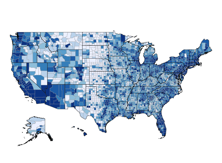
This is such a cool package, but the maps look completely unpresentable without decent projections! I know it’s something that’s been brought up before in the comments of the blog and that it’s a complicated issue, but whenever I see these posts on R-bloggers I think “ooh, that looks so great, I wish I could use it but I couldn’t show those maps to anyone so distorted”.

    Ari Lamstein says June 12, 2015

    Gregor, thanks for taking the time to comment. You can easily add any projection to any map that choroplethr produces by adding ggplot2’s coord_map() – literally just type “coord_map()”. I haven’t added a default projection to choroplethr yet for two reasons

    1. It looks like ggplot2 has a bug for projections on world maps.

    2. For all US maps I would like to use the Albers projection, which is what I believe the US Census Bureau uses. But I’m not sure what parameters I should provide to it. Also, should those pamaters change for the insets of Alaska and Hawaii, and zooms of small regions such as San Francisco above? Ideally I would not be making up numbers myself to give to it, but would use some generally accepted values. But I haven’t found a source for that yet.

    The reason I don’t manually add a projection to the maps above is that I wanted to focus on the code. I could add simply add “+ coord_map()” myself, but I think that it would just be masking the fact that I haven’t satisfactorily answered (2) myself, and incorporated it elegently into the package.

    If you can point me in the direction of answering (2) above, please let me know.

      Gregor Thomas says June 12, 2015

      That’s great! I was under the impression that there was some conflict with `coord_map`. Unfortunately I can’t help with 2, I don’t know much about projections.

      IMHO, you should add some projections manually in your blog posts… if you show the code and mention it in the text you’re not hiding anything, and it would make the demo results *much* more appealing.

        Ari Lamstein says June 12, 2015

        Gregor, thanks for the feedback. I have updated this post based on your feedback, and will follow your advice for subsequent posts as well.

          Gregor Thomas says June 16, 2015

          Looks beautiful!

        Ari Lamstein says June 16, 2015

        Thanks! I think that you will like Thursday’s post 🙂

Comments are closed